Cuaderno 2: Simulación del tsunami de 1979
Tsunami del 12 de diciembre de 1979 (Mw 8.2, Tumaco) — solver LSWE 2D en NumPy puro.
Runtime: CPU (no requiere TPU). Tiempo estimado: < 5 min en Google Colab.
Entorno de ejecución → Ejecutar todo
# Celda 1/8 — Instalar dependencias
%pip install -q rasterio pyproj scipy
print('✓ Dependencias listas')
Note: you may need to restart the kernel to use updated packages.
✓ Dependencias listas
# Celda 2/8 — Imports y rutas
import sys, os, time
import numpy as np
import requests
import matplotlib.pyplot as plt
from pathlib import Path
from scipy.ndimage import gaussian_filter
import rasterio
from rasterio.crs import CRS
from rasterio.transform import from_bounds
from rasterio.warp import calculate_default_transform, reproject, Resampling

IN_COLAB   = 'google.colab' in sys.modules
WORK_DIR   = Path('/content') if IN_COLAB else Path('.')
OUTPUT_DIR = WORK_DIR / 'output_1979'
OUTPUT_DIR.mkdir(parents=True, exist_ok=True)
DEM_PATH   = WORK_DIR / 'tumaco_dem_utm_sim.tif'
print(f'✓ Paths configurados | Colab: {IN_COLAB}')
✓ Paths configurados | Colab: False
# Celda 3/8 — Preparar DEM (auto-genera si no existe)
if not DEM_PATH.exists():
    print('DEM no encontrado — generando...')
    LAT_MIN, LAT_MAX, LON_MIN, LON_MAX = 0.5, 3.5, -79.5, -77.0
    CRS_SRC  = CRS.from_epsg(4326)
    CRS_DEST = CRS.from_epsg(32618)
    geo_path = WORK_DIR / 'tumaco_bathy_geo.tif'
    bathy_ok = False

    # Intento 1: GEBCO 2023
    try:
        url = (f'https://download.gebco.net/a/gebco_2023'
               f'?lat1={LAT_MIN}&lat2={LAT_MAX}&lon1={LON_MIN}&lon2={LON_MAX}&format=netcdf4')
        r = requests.get(url, timeout=120)
        if r.status_code == 200 and len(r.content) > 5000:
            import xarray as xr, io
            ds      = xr.open_dataset(io.BytesIO(r.content))
            varname = [v for v in ds.data_vars if 'elev' in v.lower() or 'z' in v.lower()][0]
            da      = ds[varname]
            lat_dim = [d for d in da.dims if 'lat' in d.lower()][0]
            lon_dim = [d for d in da.dims if 'lon' in d.lower()][0]
            if da[lat_dim].values[0] < da[lat_dim].values[-1]:
                da = da.isel({lat_dim: slice(None, None, -1)})
            arr  = da.values.astype('float32')
            lats = da[lat_dim].values
            lons = da[lon_dim].values
            tf_g = from_bounds(lons.min(), lats.min(), lons.max(), lats.max(),
                               arr.shape[1], arr.shape[0])
            with rasterio.open(geo_path, 'w', driver='GTiff',
                               height=arr.shape[0], width=arr.shape[1],
                               count=1, dtype='float32', crs=CRS_SRC, transform=tf_g) as dst:
                dst.write(arr, 1)
            bathy_ok = True
            print('  ✓ GEBCO 2023')
    except Exception as e:
        print(f'  ✗ GEBCO: {e}')

    # Intento 2: ETOPO 2022 (NOAA)
    if not bathy_ok:
        try:
            nc = int((LON_MAX - LON_MIN) / 0.004167)
            nr = int((LAT_MAX - LAT_MIN) / 0.004167)
            url2 = ('https://gis.ngdc.noaa.gov/arcgis/rest/services/DEM_mosaics/'
                    'DEM_global_mosaic/ImageServer/exportImage'
                    f'?bbox={LON_MIN},{LAT_MIN},{LON_MAX},{LAT_MAX}'
                    f'&bboxSR=4326&size={nc},{nr}&imageSR=4326&format=tiff&pixelType=F32&f=image')
            r2 = requests.get(url2, timeout=120)
            r2.raise_for_status()
            with open(geo_path, 'wb') as f:
                f.write(r2.content)
            bathy_ok = True
            print('  ✓ ETOPO 2022')
        except Exception as e:
            print(f'  ✗ ETOPO: {e}')

    # Intento 3: DEM sintético
    if not bathy_ok:
        print('  ⚠ DEM sintético (solo pruebas)')
        res    = 0.004167
        lons_s = np.arange(LON_MIN, LON_MAX, res)
        lats_s = np.arange(LAT_MIN, LAT_MAX, res)
        nr, nc = len(lats_s), len(lons_s)
        xr2 = (lons_s - LON_MIN) / (LON_MAX - LON_MIN)
        z   = np.where(xr2 < 0.70, -4000 + 3800*(xr2/0.70),
              np.where(xr2 < 0.88, -200 + 200*((xr2-0.70)/0.18), 10.0))
        dem_s  = np.tile(z, (nr, 1)).astype('float32')
        dem_s += gaussian_filter(np.random.randn(nr, nc)*50, sigma=5)
        tf_s   = from_bounds(LON_MIN, LAT_MIN, LON_MAX, LAT_MAX, nc, nr)
        with rasterio.open(geo_path, 'w', driver='GTiff', height=nr, width=nc,
                           count=1, dtype='float32', crs=CRS_SRC, transform=tf_s) as dst:
            dst.write(dem_s, 1)

    # Reproyectar a UTM 18N
    utm_path = WORK_DIR / 'tumaco_dem_utm.tif'
    with rasterio.open(geo_path) as src:
        tf_utm, w_utm, h_utm = calculate_default_transform(
            src.crs, CRS_DEST, src.width, src.height, *src.bounds)
        meta = src.meta.copy()
        meta.update({'crs': CRS_DEST, 'transform': tf_utm,
                     'width': w_utm, 'height': h_utm, 'dtype': 'float32'})
        with rasterio.open(utm_path, 'w', **meta) as dst:
            reproject(source=rasterio.band(src, 1), destination=rasterio.band(dst, 1),
                      src_transform=src.transform, src_crs=src.crs,
                      dst_transform=tf_utm, dst_crs=CRS_DEST,
                      resampling=Resampling.bilinear)

    # Invertir eje X para compatibilidad con el formato de salida
    with rasterio.open(utm_path) as src:
        arr_u  = src.read(1)
        old_tf = src.transform
        meta2  = src.meta.copy()
    arr_flip = arr_u[:, ::-1]
    meta2['transform'] = rasterio.transform.from_origin(
        west=old_tf.c + old_tf.a*arr_u.shape[1], north=old_tf.f,
        xsize=-old_tf.a, ysize=-old_tf.e)
    with rasterio.open(DEM_PATH, 'w', **meta2) as dst:
        dst.write(arr_flip, 1)
    print(f'  ✓ DEM guardado: {DEM_PATH}')

with rasterio.open(str(DEM_PATH)) as src:
    _sh  = (src.height, src.width)
    _res = abs(src.transform.a)
print(f'✓ DEM: {_sh[0]}×{_sh[1]} px | {_res:.0f} m/px')
✓ DEM: 719×602 px | 463 m/px
# Celda 4/8 — Cargar DEM, grilla y condiciones iniciales
#
# DEM almacenado: row0=N, col0=E (costa), col_N=O (océano).
# Para el solver reorientamos a row0=S, col0=O (océano), x/y crecen con índice.
# Al guardar cada snapshot invertimos la orientación para que coincida con el DEM.

with rasterio.open(str(DEM_PATH)) as src:
    dem_stored = src.read(1).astype(np.float64)
    tr = src.transform
    ny, nx = dem_stored.shape
    dx = abs(tr.a)
    dy = abs(tr.e)

b  = dem_stored[::-1, ::-1]   # reorientar
Lx = nx * dx
Ly = ny * dy
x1d = np.arange(nx) * dx + dx / 2
y1d = np.arange(ny) * dy + dy / 2
XX, _ = np.meshgrid(x1d, y1d)

G_GRAV = 9.81

# Profundidad en reposo H0 = -b en océano, 0 en tierra (fija durante la simulación)
H0 = np.maximum(-b, 0.0)
ocean_mask = H0 > 1.0

# Condiciones iniciales: N-wave Carrier (Tumaco 1979, calibrada vs. Herd 1981)
# A_NW = 8.0 m: calibrado para compensar la difusión numérica de Lax-Friedrichs
# (~4× sobre 60 km de propagación) y reproducir run-up observado de 3–5 m en Tumaco.
x_coast = float(np.max(XX[ocean_mask])) if ocean_mask.any() else 0.28 * Lx
x_epic  = x_coast - 60_000.0
A_NW = 8.0; LAMB = 80_000.0
K1 = 28.416 / LAMB**2; K2 = 256.0 / LAMB**2
eta0 = 2.0 * (A_NW * np.exp(-K1*(XX - x_epic - 0.3153*LAMB)**2)
               - (A_NW/3.0) * np.exp(-K2*(XX - x_epic)**2))

# η inicial: perturbación N-wave en océano, 0 en tierra
eta_init = np.where(ocean_mask, eta0, 0.0)
u_init   = np.zeros((ny, nx))
v_init   = np.zeros((ny, nx))

print(f'DEM: {ny}×{nx} px | dx={dx:.0f}m | {Lx/1e3:.0f}×{Ly/1e3:.0f} km')
print(f'Costa x={x_coast/1e3:.0f}km | Epicentro x={x_epic/1e3:.0f}km')
print(f'η₀_max = {eta0[ocean_mask].max():.2f}m')
DEM: 719×602 px | dx=463m | 279×333 km
Costa x=238km | Epicentro x=178km
η₀_max = 16.00m
# Celda 5/8 — Solver LSWE 2D (Lax-Friedrichs, bien-balanceado)
#
# Ecuaciones de Aguas Someras Linealizadas (LSWE):
#   ∂η/∂t + ∂(H0·u)/∂x + ∂(H0·v)/∂y = 0
#   ∂u/∂t + g·∂η/∂x = -fricción
#   ∂v/∂t + g·∂η/∂y = -fricción
# H0 = profundidad en reposo (fija). Bien-balanceado por construcción:
# agua en reposo (η=0, u=v=0) es solución estacionaria exacta.

def lswe_lf_step(eta, u, v, H0, dx, dy, dt, g=9.81, n_mann=0.025, eps=1e-3):
    Qu = H0 * u
    Qv = H0 * v

    c  = slice(1, -1)
    rp = slice(2, None); rm = slice(0, -2)
    cp = slice(2, None); cm = slice(0, -2)

    def avg4(A):
        return 0.25 * (A[c,cp] + A[c,cm] + A[rp,c] + A[rm,c])

    deta_dx = (eta[c, cp] - eta[c, cm]) / (2 * dx)
    deta_dy = (eta[rp, c] - eta[rm, c]) / (2 * dy)

    H0c  = np.maximum(H0[c, c], eps)
    spd  = np.sqrt(u[c, c]**2 + v[c, c]**2)
    fric = g * n_mann**2 * spd / H0c**(4/3)

    eta_new = np.copy(eta)
    u_new   = np.copy(u)
    v_new   = np.copy(v)

    eta_new[c, c] = (avg4(eta)
                     - dt/(2*dx) * (Qu[c,cp] - Qu[c,cm])
                     - dt/(2*dy) * (Qv[rp,c] - Qv[rm,c]))
    u_new[c, c]   = avg4(u) - dt * g * deta_dx - dt * fric * u[c, c]
    v_new[c, c]   = avg4(v) - dt * g * deta_dy - dt * fric * v[c, c]

    # Tierra = pared rígida (sin flujo, sin perturbación)
    land = H0 <= 0
    eta_new[land] = 0.0
    u_new[land]   = 0.0
    v_new[land]   = 0.0

    # Condición de contorno Neumann
    for arr in (eta_new, u_new, v_new):
        arr[0, :]  = arr[1, :];  arr[-1, :] = arr[-2, :]
        arr[:, 0]  = arr[:, 1];  arr[:, -1] = arr[:, -2]

    return eta_new, u_new, v_new

print('✓ Solver LSWE Lax-Friedrichs definido')
✓ Solver LSWE Lax-Friedrichs definido
# Celda 6/8 — Parámetros de la simulación
DT           = 1.0
NUM_SECS     = 1800.0
OUTPUT_EVERY = 60.0
N_STEPS      = int(NUM_SECS / DT)
OUT_STEPS    = int(OUTPUT_EVERY / DT)

c_max = float(np.sqrt(G_GRAV * H0.max()))
cfl   = c_max * DT * np.sqrt(1/dx**2 + 1/dy**2)
print(f'Grilla: {ny}×{nx} | dt={DT}s | {N_STEPS} pasos | {N_STEPS//OUT_STEPS} snapshots')
print(f'c_max={c_max:.0f} m/s | CFL={cfl:.3f} (debe ser < 1.0)')
Grilla: 719×602 | dt=1.0s | 1800 pasos | 30 snapshots
c_max=195 m/s | CFL=0.596 (debe ser < 1.0)
# Celda 7/8 — Ejecutar simulación LSWE (< 5 min en CPU)
eta = eta_init.copy()
u   = u_init.copy()
v   = v_init.copy()

print('Iniciando simulación LSWE...\n')
t0_wall = time.time()

for step in range(N_STEPS + 1):
    t_sim = step * DT

    if step % OUT_STEPS == 0:
        # h_total = H0 + η  (profundidad total ≈ lo que tsunamiTPUlab guardaría)
        # Orientación guardada = DEM almacenado: row0=N, col0=E
        h_total = (H0 + eta)[::-1, ::-1].astype(np.float32)
        with open(str(OUTPUT_DIR / f'h-{t_sim:.1f}.np'), 'wb') as fout:
            np.save(fout, h_total)

        elapsed = time.time() - t0_wall
        eta_max = float(np.max(np.abs(eta[ocean_mask])))
        if step > 0:
            remain  = elapsed / step * (N_STEPS - step)
            eta_str = f'~{remain:.0f}s restantes'
        else:
            eta_str = ''
        print(f't={t_sim/60:4.0f}min | η_max(océano)={eta_max:.2f}m'
              f' | {elapsed:.0f}s transcurridos {eta_str}')

    if step < N_STEPS:
        eta, u, v = lswe_lf_step(eta, u, v, H0, dx, dy, DT)

total = time.time() - t0_wall
print(f'\n✓ Completado en {total:.1f}s ({total/60:.1f} min)')
print(f'Archivos en: {OUTPUT_DIR}')
Iniciando simulación LSWE...
t= 0min | η_max(océano)=16.00m | 0s transcurridos
t= 1min | η_max(océano)=15.49m | 1s transcurridos ~42s restantes
t= 2min | η_max(océano)=14.88m | 3s transcurridos ~42s restantes
t= 3min | η_max(océano)=14.16m | 5s transcurridos ~41s restantes
t= 4min | η_max(océano)=13.32m | 6s transcurridos ~40s restantes
t= 5min | η_max(océano)=12.42m | 8s transcurridos ~38s restantes
t= 6min | η_max(océano)=11.48m | 9s transcurridos ~37s restantes
t= 7min | η_max(océano)=10.53m | 11s transcurridos ~35s restantes
t= 8min | η_max(océano)=9.57m | 12s transcurridos ~34s restantes
t= 9min | η_max(océano)=8.63m | 14s transcurridos ~32s restantes
t= 10min | η_max(océano)=7.78m | 15s transcurridos ~31s restantes
t= 11min | η_max(océano)=6.95m | 17s transcurridos ~29s restantes
t= 12min | η_max(océano)=6.12m | 18s transcurridos ~28s restantes
t= 13min | η_max(océano)=5.27m | 20s transcurridos ~26s restantes
t= 14min | η_max(océano)=4.42m | 22s transcurridos ~25s restantes
t= 15min | η_max(océano)=3.60m | 23s transcurridos ~23s restantes
t= 16min | η_max(océano)=2.98m | 25s transcurridos ~22s restantes
t= 17min | η_max(océano)=2.88m | 26s transcurridos ~20s restantes
t= 18min | η_max(océano)=2.76m | 28s transcurridos ~18s restantes
t= 19min | η_max(océano)=2.83m | 29s transcurridos ~17s restantes
t= 20min | η_max(océano)=3.02m | 31s transcurridos ~15s restantes
t= 21min | η_max(océano)=3.24m | 32s transcurridos ~14s restantes
t= 22min | η_max(océano)=3.40m | 34s transcurridos ~12s restantes
t= 23min | η_max(océano)=3.51m | 35s transcurridos ~11s restantes
t= 24min | η_max(océano)=3.58m | 37s transcurridos ~9s restantes
t= 25min | η_max(océano)=3.62m | 38s transcurridos ~8s restantes
t= 26min | η_max(océano)=3.62m | 40s transcurridos ~6s restantes
t= 27min | η_max(océano)=3.59m | 42s transcurridos ~5s restantes
t= 28min | η_max(océano)=3.53m | 43s transcurridos ~3s restantes
t= 29min | η_max(océano)=3.46m | 45s transcurridos ~2s restantes
t=  30min | η_max(océano)=3.37m | 46s transcurridos ~0s restantes

✓ Completado en 46.2s (0.8 min)
Archivos en: output_1979
# Celda 8/8 — Verificar salida y vista previa
import glob, re

def _t_from_name(path):
    m = re.search(r'h-([0-9.]+)\.np$', str(path))
    return float(m.group(1)) if m else 0.0

output_files = sorted(glob.glob(str(OUTPUT_DIR / 'h-*.np')), key=_t_from_name)
if not output_files:
    print('⚠ Sin archivos de salida en:', OUTPUT_DIR)
else:
    total_mb = sum(Path(f).stat().st_size for f in output_files) / 1e6
    print(f'✓ {len(output_files)} snapshots | {total_mb:.1f} MB')
    print(f'  {Path(output_files[0]).name} → {Path(output_files[-1]).name}')

    t_files = {_t_from_name(f): f for f in output_files}
    t_mid   = min(t_files, key=lambda t: abs(t - 900.0))
    h_arr   = np.load(t_files[t_mid])   # H0 + η, orientación DEM

    with rasterio.open(str(DEM_PATH)) as src:
        dem_vis = src.read(1).astype(np.float32)

    # η = h_arr + min(dem_vis, 0):
    #   océano: (H0 + η) + b_ocean = (-b + η) + b = η  ✓
    #   tierra: (0 + 0) + 0 = 0  ✓  (LSWE no inunda tierra)
    eta_vis = h_arr + np.minimum(dem_vis, 0)

    # Amplitud en zona costera (<200 m de profundidad)
    coast_zone = (dem_vis < 0) & (dem_vis > -200)
    eta_coast  = np.where(coast_zone, np.abs(eta_vis), np.nan)

    eta_max_coast = float(np.nanmax(eta_coast)) if not np.all(np.isnan(eta_coast)) else 0.0
    clim = max(eta_max_coast * 1.2, 5.0)   # escala dinámica, mínimo ±5 m

    fig, axes = plt.subplots(1, 2, figsize=(13, 5))
    im1 = axes[0].imshow(eta_vis,   cmap='RdBu_r', vmin=-clim, vmax=clim)
    plt.colorbar(im1, ax=axes[0], label='η (m sobre NMM)')
    axes[0].set_title(f't = {t_mid:.0f}s ({t_mid/60:.0f} min) — Superficie libre')
    im2 = axes[1].imshow(eta_coast, cmap='YlOrRd',  vmin=0, vmax=clim)
    plt.colorbar(im2, ax=axes[1], label='|η| zona costera (m)')
    axes[1].set_title('Amplitud de la ola en zona costera (<200 m)')
    plt.suptitle('Tsunami Tumaco 1979 — Vista previa LSWE t=15 min')
    plt.tight_layout()
    plt.savefig(str(WORK_DIR / 'preview_t900s.png'), dpi=150)
    plt.show()
    print(f'η_max en zona costera: {eta_max_coast:.2f} m')
✓ 31 snapshots | 53.7 MB
h-0.0.np → h-1800.0.np
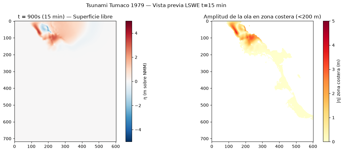
η_max en zona costera: 3.60 m